Steps to Derive k and Assemble into K

Figure 1 is a flowchart illustrating the sequence for computing the stiffness matrix of a simple problem (the concept is similar to more complex problems). Computing the stiffness matrix involves two main steps:

1. Derive local stiffness matrices (k)
2. Assemble k into K, the global stiffness matrix

Matrix Methods: Direct vs. Iterative

Direct vs. Iterative methods
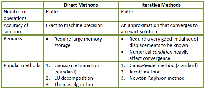
The two approaches available for solving global stiffness matrix (K) in FEM are:

Implications on FEA solver

• For linear simulation e.g. KU = f , Gaussian elimination can be applied directly
• For nonlinear simulation e.g. K(u)U=f, stiffness is dependent on displacements (u). Therefore an iterative method must be used.

See also
The role of matrix solution in the FEM process

What is Meshing?

Meshing involves:

1. discretisation of a continuum into finite number of elements
2. defining element type (determined by shape functions)
3. nodal connectivity

A finite element mesh adapted from Dr TE Kendon's research page

Traditionally, meshing is performed by human user. Automatic meshing technologies are becoming more readily available and user friendly in FEA pre-processors as the competition in the FEA software market gets fierce than ever.

Also read

The role of meshing in FEM

Virtual Work and Weak Formulation

Weak formulations (a.k.a. variational formulations) of partial differential equations (PDEs) are hugely important in the FEM as they enable the concepts of linear algebra in the analysis of PDEs. This concept transform PDEs into sets of linear equations (a matrix) that can eventually be manipulated and inverted using standard matrix methods.

Transforming an equation from strong to weak form requires the use of virtual function, and hence the name Principle of Virtual Work.

Also read
A few worked examples (external pdf)
The role of the Principle of Virtual Work in FEM

Boundary Conditions (BCs) vs. Displacement BCs in FEM

This post aims to address the question that arises when one cannot distinguish between boundary conditions (BCs) and displacement BCs in the flowchart of FEM process.

Since FEM is all about solving the FE equation in matrix form, we approach this question using the classic FE equation of a linear elastic problem, KU = f. Let us assume it expands to look like Figure 1:

Figure 1: FE Equation of a linear elastic problem, KU = f

We can now interpret the difference between BCs and displacement BCs from the physical and mathematical perspectives:

Steps in FEM: An Overview

Figure 1 is a flowchart illustrating the FEM process for a linear static problem (the concept is similar to more complex problems):

Figure 1: A finite element method process for solving linear static problems (Click to enlarge)

Brief explaination of the different stages in Figure 1: